In order to use LecChip (lectin microarray) data to identify the structure of glycan structures, cell types, etc., it is effective to use Deep learning on a large amount of data.
The preparations required for this work are as follows.
Python(Anaconda3 is used below)
Tensorflow
Keras
First of all, you need to install these software on your PC and create an environment.
Our product “SA/DL Easy” eliminates such the hassle preparation in advance and allows you to configure Deep learning networks with just a click of a mouse.
Using SA/DL Easy, you can easily enjoy the world for Deep learning without writing scripts like the one below.
When executing the following scripts on your PC, please make sure if the path of the Python script is saved, the path of the saved input data, the path of the folder where the learning results and test results are correctly specified.
———————————————————————————————
# An example of Deep learning Python Script for identifing glycan structures, cell types, etc. using LecChip data.
from __future__ import print_function
import numpy as np
import csv
import pandas
from keras.datasets import mnist
from keras.models import Sequential
from keras.layers.core import Dense, Dropout, Activation
from keras.optimizers import RMSprop
from keras.utils import np_utils
from make_tensorboard import make_tensorboard
np.random.seed(1671) # for reproducibility
# network and training
NB_EPOCH = 100 # how many times you want to let them learn.
BATCH_SIZE = 2 # divide the dataset into several subsets
VERBOSE = 1
NB_CLASSES = 2 # final output number
OPTIMIZER = RMSprop() # optimizer
N_HIDDEN = 45 # number of nodes in the hidden layer is set to 45 here according to the number of lectins used in LecChip.
VALIDATION_SPLIT = 0.2 # percentage of the training data used as test data
DROPOUT = 0.3
LECTINS = 45
def drop(df):
return df[pandas.to_numeric(df.iloc[:, 2], errors=’coerce’).notnull()]
# data is normalized so that the maximum value is 1.
def normalize_column(d):
dmax = np.max(d)
dmin = np.min(d)
return (np.log10(d + 1.0) – np.log10(dmin + 1.0)) / \
(np.log10(dmax + 1.0) – np.log10(dmin + 1.0))
def normalize(data):
return np.apply_along_axis(normalize_column, 0, data)
# The input data should be in CSV file format
df1 = drop(pandas.read_csv(r’c:\Users\Masao\Anaconda3\DL_scripts\cell.csv’)).reset_index(drop=True)
X_train = normalize(df1.iloc[:, 2:].astype(np.float64))
family_column = df1.iloc[:, 1]
family_list = sorted(list(set(family_column)))
Y_train = np.array([family_list.index(f) for f in family_column])
df2 = drop(pandas.read_csv(r’c:\Users\Masao\Anaconda3\DL_scripts\cell_test.csv’)).reset_index(drop=True)
X_test = normalize(df2.iloc[:, 2:].astype(np.float64))
familyt_column = df2.iloc[:, 1]
familyt_list = sorted(list(set(familyt_column)))
Y_test = np.array([familyt_list.index(f) for f in familyt_column])
print(X_train.shape[0], ‘train samples’)
print(X_test.shape[0], ‘test samples’)
# convert class vectors to binary class matrices
Y_train = np_utils.to_categorical(Y_train, NB_CLASSES)
Y_test = np_utils.to_categorical(Y_test, NB_CLASSES)
print(X_train)
print(Y_train)
print(X_test)
print(Y_test)
# An example of neural network configuration
# 2 hidden layers
# Input is LecChip data (using 45 lectins)
# The final layer is activated with softmax
model = Sequential()
model.add(Dense(N_HIDDEN, input_shape=(LECTINS,)))
model.add(Activation(‘relu’))
model.add(Dropout(DROPOUT))
model.add(Dense(N_HIDDEN))
model.add(Activation(‘relu’))
model.add(Dropout(DROPOUT))
model.add(Dense(NB_CLASSES))
model.add(Activation(‘softmax’))
model.summary()
# to visualize the learning and the test results with Tensorboard
callbacks = [make_tensorboard(set_dir_name=’Glycan_Profile’)]
model.compile(loss=’categorical_crossentropy’,
optimizer=OPTIMIZER,
metrics=[‘accuracy’])
model.fit(X_train, Y_train,
batch_size=BATCH_SIZE, epochs=NB_EPOCH,
callbacks=callbacks,
verbose=VERBOSE, validation_split=VALIDATION_SPLIT)
score = model.evaluate(X_test, Y_test, verbose=VERBOSE)
print(“\nTest score:”, score[0])
print(‘Test accuracy:’, score[1])
————————————————————————————
# Python Script for using Tensorboard
# -*- coding: utf-8 -*-
from __future__ import absolute_import
from __future__ import unicode_literals
from time import gmtime, strftime
from keras.callbacks import TensorBoard
import os
def make_tensorboard(set_dir_name=”):
ymdt = strftime(“%a_%d_%b_%Y_%H_%M_%S”, gmtime())
directory_name = ymdt
log_dir = set_dir_name + ‘_’ + directory_name
os.mkdir(log_dir)
tensorboard = TensorBoard(log_dir=log_dir, write_graph=True, )
return tensorboard
————————————————————————————
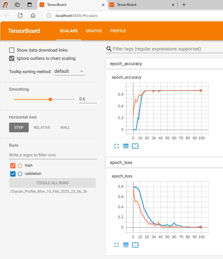
To visualize the learning and test results,
run $ make_tensorboard.py,
run $ tensorboard –logdir=./Glycan_Profile_Mon_10_Feb_2025_23_06_26 (./folder where data is recorded),
and access http://localhost:6006/ with your browser.
(base) PS C:\Users\masao\Anaconda3\DL_Scripts> python make_tensorboard.py
Using TensorFlow backend.
(base) PS C:\Users\masao\Anaconda3\DL_Scripts> tensorboard –logdir=./Glycan_Profile_Mon_10_Feb_2025_23_06_26
Serving TensorBoard on localhost; to expose to the network, use a proxy or pass –bind_all
TensorBoard 2.0.2 at http://localhost:6006/ (Press CTRL+C to quit)
—————————————————————————————————-
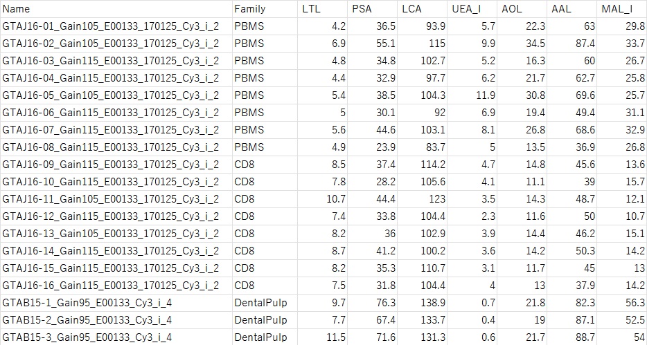
LecChip data is in CSV format as shown below.
From the left, the sample name, family name (this will be the training data), and numerical values of various lectins are listed.
—————————————————————————————————-
After the training, you should save the model.
If the model was saved, it could be restored, and unknown data can be given to make predictions.
Those scripts will be uploaded separately for your information.


